The LP Calculator is a free online tool. So, it provides the best optimum solution given the restrictions. Then, any online LP calculator tool accelerates computations. Also, it presents the best optimum solution for the supplied objective functions with the system of linear constraints in a fraction of a second. Then, LP is also popular as Linear Optimization. Also, this is a subset of mathematical programming. It is also popular as mathematical optimization.

So, it is a method for providing the optimal solution or output in a mathematical model. Then, in the procedure, We can see variable values of a particular objective function, such as maximize or minimize. Also, constraints establish the range in LP. On the other hand, the objective function defines the quantity to be optimized. Then, LP is most commonly employed in mathematics. But we can apply it in a variety of fields of study.

In this article, we are talking about this calculator. So, keep reading to know more about it.

Linear Programming Problem Calculator

So, LP is the most effective optimization approach for solving objective functions. Also, it provides linear variables and linear constraints. Then, it also gives the best solution to a given linear issue. Also, the primary goal of the approach is to determine the values of variables required to maximize or decrease the target function.

On the other hand, we can use it to describe the quantity or value that should be optimized. So, we can use constraints to define the variable’s range. Also, it has four major components. So, these are the goal function, constraints, data, and the decision variable. Then, all of these elements must be present in order to solve the challenge.

Linear Programming Problem Calculator with steps

So, now that you know what it is, let’s look at how to utilize the LP problem calculator.

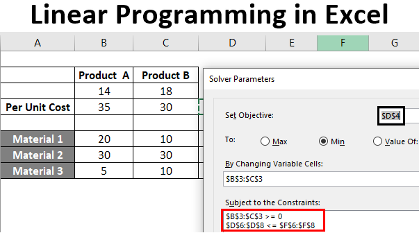
It is essentially a free online calculator. It gives the most efficient and optimal solution for specified limitations in a matter of seconds. To utilize it, take these steps:

• First, enter constraints and the goal function in the appropriate input fields.
• Then, in the offered tool, click the submit button to find the best solution to the linear issue.
• Then, a new window will open. So, it displays the best solution to the specified issue in the form of a graph.

Also, these are the fundamental steps to utilizing this calculator. When utilizing a LP calculator, you should pick whether to maximize or minimize the input for the specified linear issue. The Maximizing calculator is a calculator that solely provides maximization capabilities to solve a linear issue. However, if you solely use minimizing functionality to compute the issue, it might be deemed a Minimization calculator.

Linear Programming Problem Calculator solver online

Furthermore, issues may be addressed using the TI 84 Plus LP Calculator. It is a strategy for solving and determining the maximum and minimum values of a multivariable and objective function that is bound by inequalities in the system.

However, you may solve these inequalities using the TI 84 Plus LP Calculator. It is based on the principle that if the issue contains a system of inequalities, the objective function should be evaluated at the point of intersection where the smallest value is the minimum value of the function and the biggest value is the maximum value of the function. Inequalities might be resolved in this manner.

Follow these procedures to get the maximum and minimum values for a given linear problem using the TI-84 Plus:

• Plot the graph for the constraint system specified in the linear problem.
• Determine the intersection region and then graph the intersection region.
• After that, discover junction points in the region and save them in the graph.
• Display the saved intersection points in the TI-84 Plus calculator.
• Make a list of inequalities using the intersection points shown.

Determine a formula for your function and then use it to determine the inequality entries.

Then, press E to evaluate the function, and you’ll obtain the maximum and lowest values from the inequality system.

Linear Programming Problem Calculator Uses

Using the above methods, linear problems may be solved with a LP calculator, such as the TI-84 plus. A LP calculator with three variables is another tool available for solving linear problems using a different technique. When you have more than one linear equation or three linear equations to solve a problem with three provided variables, you can use this calculator. To solve three linear equations for a particular linear issue, simply enter all three equations into this tool and you will receive your answer.

When you use an LP calculator to solve a problem, it will give you a direct solution of maximization or minimization. However, a minimization calculator is accessible if you wish to identify a minimum element of a data set for a linear issue step by step. Similarly, you may use a maximize calculator to iteratively determine the maximum element of a data collection for a specified linear problem. This will help you comprehend linear issues more thoroughly.

Linear Programming Problem Calculator with graph

Graphical Method: Because LP models are so important in many sectors, several different types of algorithms have been created throughout the years to solve them. The Simplex technique, the Hungarian approach, and others are well-known examples. The graphical technique is one of the most fundamental ways for dealing with a LP problem.

Read Also: The Molar Mass of Oxygen Molecule – Definition, Formula, and Example

In principle, this strategy works for practically all sorts of issues, but it becomes increasingly difficult to solve as the number of choice factors and restrictions rises. As a result, we’ll demonstrate it in a basic instance with only two variables. So, let us begin with the graphical way.

Linear Programming Problem Calculator Graphical method

We will first go over the algorithm’s steps:

Step 1: Create the LP (LP) problem.

In the preceding part, we discussed the mathematical formulation of an LP issue. This is the most important phase since all following steps are dependent on our analysis here.

Step two: Make a graph and draw the constraint lines on it.

The graph must have ‘n’ dimensions, where ‘n’ is the number of choice variables. This should give you a sense of how difficult this phase will get as the number of choice factors rises. One must understand that one cannot envision more than three dimensions. Constrained lines are formed by connecting the horizontal and vertical intercepts given in each constraint equation.

Step 3: Determine which side of each constraint line is legitimate.

This is used to determine the domain of accessible space, which can lead to a viable solution. How do you check? An easy way is to insert the origin coordinates (0,0) into the issue and see if the objective function has a physical solution or not. If true, the valid side is the side of the constraint lines on which the origin is located. Otherwise, it’s on the opposite side.

Step 4: Determine the viable solution region

The viable solution area on the graph is the one that meets all of the restrictions. It might also be seen as the intersection of the valid areas of each constraint line. Any point in this area would yield a valid solution to our goal function.

Step 5: Draw a graph of the objective function.

Because we are working with linear equations, it will undoubtedly be a straight line. To avoid misunderstanding, it must be drawn separately from the constraint lines. Choose the constant value in the objective function equation at random to make it easily discernible.

Step 6: Determine the best spot

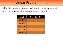
Maximum Points

An optimal point is always located on one of the feasible region’s corners. Where can I locate it? Place a ruler parallel to the objective function on the graph sheet. Make care to maintain this ruler’s orientation in space. We simply require the direction of the goal function’s straight line. Begin at the far left corner of the graph and work your way towards the origin.

Find the point of contact of the ruler with the feasible region that is closest to the origin if the purpose is to minimize the objective function. This is the best moment to minimize the function.

Find the point of contact of the ruler with the feasible region that is the farthest from the origin if the purpose is to maximize the objective function. This is the best location to maximize the function.

Linear Programming Problem Calculator transportation

A business wants to reduce the cost of transporting a product from two plants to five separate clients. Every manufacturing has a limited supply, and every consumer has a specific need. How should the product be distributed by the company?

Solution

1) The variables are the amount of items shipped from each facility to customers. In worksheet Transport1, these are labeled Products shipped.

2) Using the Assume Non-Negative option, the logical constraint is Products shipped >= 0.

The other two limitations are Total received >= Demand and Total shipped >= Capacity.

3) The goal is to keep costs as low as possible. Total cost is supplied to this.

Remarks

In its most basic form, this is a transportation challenge. Nonetheless, this strategy is routinely utilized to save tens of thousands of dollars each year. In worksheet Transport2, we will look at a two-level transportation problem, and in worksheet Transport3, we will look at a multi-product, two-level transportation problem.

Linear Programming Problem Calculator equation

Linear Programming Problem Calculator Equation 1

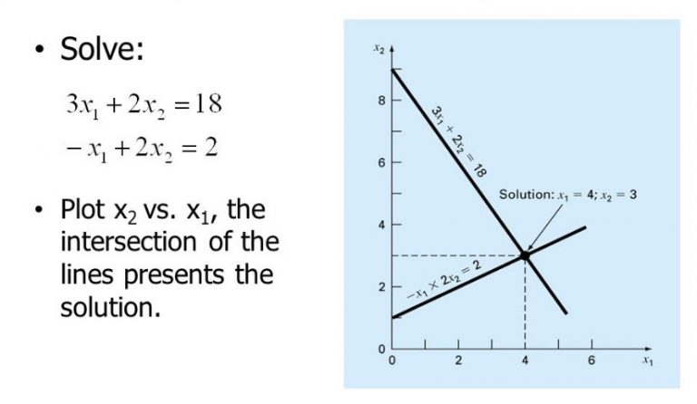
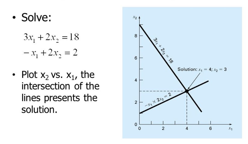
Find the feasible region for 2x+y=1000, 2x+3y=1500, x=0, y=0, as well as maximum and minimize for the objective function 50x+40y.

Answer:

In light of this, f(x,y)=50x+40y is the objective function.

The limitations are as follows:

2x+3y = 1500, x=0, y=0

2x+y=1000

y=1000-2x

2x+3y=1500

Then, 3y=1500-2x

Then, y=(1500-2x)/3

Atlast, y=500-2x/3

Now, the graph will look like this: the shaded area represents the viable region.

(0,500), (375,250), and (0,500) are the vertices (500,0).

f(x,y)=50x+40y

Replace the vertices in the objective function.

f(0,500)=50*0+40*500=20,000

Then, f(375,250)=50*375+40*250=28,750

f(500,0)=50*500+40*0=25,000

The bare minimum is (0,500)

The highest possible values are (275,250)

Linear Programming Problem Calculator Equation 2

Determine the maximum and minimum values of z = 5x + 3y under the given conditions.

x + 2y ≤ 14

3x – y ≥ 0

x – y ≤ 2

Solution:

The three inequalities show the limitations. The viable zone is the area of the plane that will be marked.

(z) = 5x + 3y is the optimization equation. You must locate the (x,y) corner locations that result in the highest and smallest values of z.

To begin, solve each inequality separately.

So, x + 2y ≤ 14 ⇒ y ≤ -(1/2)x + 7

Then, 3x – y ≥ 0 ⇒ y ≤ 3x

Then, x – y ≤ 2 ⇒ y ≥ x – 2

Now connect the lines to create a system of linear equations in order to determine the corner locations.

y = -(½) x + 7

y = 3x

We obtain the corner positions by solving the aforementioned equations (2, 6)

y = -2/x + 7

y = – 2 x

We obtain the corner positions by solving the aforementioned equations (6, 4)

3x = y

y = – 2 x

We obtain the corner positions by solving the aforementioned equations (-1, -3). The maximum and lowest values of the optimization equation for linear systems are located on the corners of the feasible zone. To obtain the best answer, just enter these three points into the equation z = 3x + 4y.

(2, 6) : z = 5(2) + 3(6) = 10 + 18 = 28

(6, 4): z = 5(6) + 3(4) = 30 + 12 = 42

(–1, –3): z = 5(-1) + 3(-3) = -5 -9 = -14

As a result, the maximum of z = 42 is found at (6, 4) while the lowest of z = -14 is found at (-1, -3).

Linear Programming Problem Calculator simplex method

One of the most prominent ways for solving LP issues is the simplex method. It is an iterative procedure to find the best practicable answer. The value of the fundamental variable is transformed in this manner to produce the greatest value for the objective function. The LP simplex technique algorithm is presented below:

Step 1: Identify a specific problem. Write the inequality restrictions and objective function, for example.

Step 2: Convert the supplied inequalities to equations by including the slack variable into each inequality statement.

Step 3: Make the first simplex tableau. In the bottom row, write the objective function. Each inequality restriction appears in its own row in this case. The issue may now be represented as an augmented matrix, which is known as the first simplex tableau.

Step 4: Find the most negative item in the bottom row, which will help you find the pivot column. The strongest negative item in the bottom row specifies the largest coefficient in the goal function, which will aid us in increasing the objective function’s value as quickly as possible.

Step 5: Determine the quotients. To find the quotient, divide the items in the far right column by the entries in the first column (excluding the bottom row). The least quotient identified the row.

The pivot element will be the row identified in this step and the element identified in this step.

Step 6: Use pivoting to ensure that all other items in the column are zero.

Step 7: Stop the procedure if there are no negative entries in the bottom row. Otherwise, proceed to step 4.

Step 8: Finally, find the solution that corresponds to the final simplex tableau.

Linear Programming Problem Calculator application

Various sectors make extensive use of optimization and LP. So, people used LP in the manufacturing and service industries. In this part, we will look at the numerous applications of LP.

Manufacturing sectors employ LP to study their supply networks. Manufacturing industries try to be as efficient as possible in their operations. A LP model can advise a firm on modifications to its storage arrangement, personnel, and production bottlenecks. Watch this video for a more in-depth look at a Warehouse case study from Cequent, a firm situated in the United States. People used LP to maximize shelf space in organized retail.

With so many items on the market today, it is critical to understand what buyers want. Big Bazaar, Walmart, Hypercity, Reliance, and other retailers make extensive use of optimization. The goods in the store are carefully positioned based on how people shop. Customers should be able to simply identify and pick the relevant goods. This is not achievable due to constraints such as limited shelf space and a diverse product line.

We can use optimization to save costs in addition to optimizing delivery routes.

That is a variation on the well-known traveling salesman dilemma. We can use optimization to discover the most efficient path for an industry. It requires several salesmen visiting multiple cities. FedEx, Amazon, and other companies use a clustering and greedy algorithm to calculate delivery routes.

Linear Programming Problem Calculator Objective

Our objective is to cut operational expenses and time. Optimizations are also employed in Machine Learning. The core of supervised learning is LP. By fitting a mathematical model based on the labeled input data, the system is taught to determine the values from the unknown input data.

LP, on the other hand, offers a wide range of applications. Shareholders, sports, stock markets, and other organizations use LP in the real world.

Linear Programming Problem Calculator Formulation

Step 1

So, Wheat’s entire growth area = X (in hectares)

Then, Y is the total area for cultivating barley (in hectares)

My choice factors are X and Y.

Step 2: Develop the objective function

Because the full land’s output can be sold on the market. The farmer’s goal would be to maximize his entire earnings. Net profit is shown for both wheat and barley. The farmer makes a net profit of US$50 per hectare of Wheat and US$120 per hectare of Barley.

Max Z = 50X + 120Y is our objective function.

Step 3: Document the restrictions

1. Assume the farmer has a total budget of $10,000 USD.

We are also provided the cost of growing wheat and barley per acre. We have a cap on the overall cost incurred by the farmer. As a result, our equation is: 10,000 = 100X + 200Y.

2. The next limitation is the upper limit on the total number of man-days available for the planning horizon. The total number of available man-days is 1200. The table shows the man-days per hectare for wheat and barley.

1200 = 10X + 30Y

3. The total area available for planting is the third limitation. The entire space accessible is 110 hectares. As a result, the equation becomes,

110 X + Y

Step 4: The non-negativity constraint

X and Y values will be larger than or equal to 0.

This should go without saying.

X = 0 and Y = 0

Some frequently asked questions

How do you find the optimal solution in a LP calculator?

• First, fill in the goal function and restrictions in the appropriate input fields.
• Then, to obtain the best answer, click the “Submit” button.
• Finally, in the new window, you will see the best optimum solution and the graph.

How do you find the maximum and minimum of LP?

An ideal value will occur at one of the vertices of the area indicating the set of possible solutions if a LP problem can be optimized. The greatest or lowest value of f(x,y)=ax+by+c across the set of viable solutions graphed, for example, occurs at point A,B,C,D,E, or F.

How do you find the feasible region?

The feasible region is the area of a graph that contains all of the points that fulfill all of the inequalities in a system. Graph every inequality in the system first, then the viable region. Then locate the point where all of the graphs overlap. That is the conceivable range.

Is LP hard?

LP can be solved in polynomial time, however Integer LP may be simplified to SAT, making it NP-hard (it can actually be shown to be NP complete, but this is less trivial). As a result, if PNP, LP is simpler (computationally) than ILP.

What is a LPP with an example?

(LPP) are problems. We used it to determine the best value for a given linear function. The ideal value might be either the greatest or the least. The linear function is an objective function in this context.

How do you calculate the increase?

% Increase = Increase / Original Number 100. This calculates the overall percentage change or increase. To compute a percentage decline, first determine the difference (decrease) between the two figures under consideration. Then, divide the reduction by the original number and multiply the result by 100.

What is the example of LP?

Using the graphical method, solve the following LP issue.

Minimize: Z = 5x + 4y

4x + y ≥ 40,

2x + 3y ≥ 90,

x, y ≥ 0

Solution:

Using the restrictions, we obtain the equations of the lines as 4x + y = 40 and 2x + 3y = 90.

4x + y = 40 traverses (0, 40) and (10, 0). Any point on or above this line fulfills 4x + y 40.

2x + 3y = 90 traverses (0, 30) and (45, 0). Any point on or above this line fulfills 2x + 3y ≥ 90.

Corner Points	Z = 5x + 4y
A = (45, 0)	225
B = (3, 28)	127
C = (0, 40)	160

Because the minimal value of Z is 127, B (3, 28) provides the best option.

Answer: The smallest number of Z is 127, and the best option is (3, 28)